⛴️ Winds in Chesapeake Bay#

Demonstrates pivoting, rolling averages, and wind vectors

[1]:

from datetime import datetime

import matplotlib.pyplot as plt
import polars as pl
import seaborn as sns
from herbie.toolbox import EasyMap

import synoptic

/home/blaylock/miniconda3/envs/synoptic2/lib/python3.12/site-packages/pyproj/__init__.py:89: UserWarning: pyproj unable to set database path.
  _pyproj_global_context_initialize()

[2]:

df = synoptic.TimeSeries(
    start=datetime(2017, 8, 1),
    end=datetime(2017, 8, 4),
    vars=["wind_speed", "wind_direction", "wind_gust"],
    stid=["YKRV2", "44072", "WDSV2", "CBBV2"],
).df()
df

🚚💨 Speedy delivery from Synoptic timeseries service.
📦 Received data from 4 stations.

[2]:

shape: (6_666, 20)

date_time	variable	sensor_index	is_derived	value	units	id	stid	name	elevation	latitude	longitude	mnet_id	state	timezone	elev_dem	period_of_record_start	period_of_record_end	is_restricted	is_active
datetime[μs, UTC]	str	u32	bool	f64	str	u32	str	str	f64	f64	f64	u32	str	str	f64	datetime[μs, UTC]	datetime[μs, UTC]	bool	bool
2017-08-01 00:00:00 UTC	"wind_gust"	1	false	4.02	"m/s"	23426	"YKRV2"	"York River East Rear Range Lig…	0.0	37.25	-76.3333	121	"VA"	"America/New_York"	0.0	2016-12-14 16:49:00 UTC	2023-08-16 12:54:00 UTC	false	false
2017-08-01 00:06:00 UTC	"wind_gust"	1	false	4.47	"m/s"	23426	"YKRV2"	"York River East Rear Range Lig…	0.0	37.25	-76.3333	121	"VA"	"America/New_York"	0.0	2016-12-14 16:49:00 UTC	2023-08-16 12:54:00 UTC	false	false
2017-08-01 00:12:00 UTC	"wind_gust"	1	false	3.58	"m/s"	23426	"YKRV2"	"York River East Rear Range Lig…	0.0	37.25	-76.3333	121	"VA"	"America/New_York"	0.0	2016-12-14 16:49:00 UTC	2023-08-16 12:54:00 UTC	false	false
2017-08-01 00:18:00 UTC	"wind_gust"	1	false	4.47	"m/s"	23426	"YKRV2"	"York River East Rear Range Lig…	0.0	37.25	-76.3333	121	"VA"	"America/New_York"	0.0	2016-12-14 16:49:00 UTC	2023-08-16 12:54:00 UTC	false	false
2017-08-01 00:24:00 UTC	"wind_gust"	1	false	4.47	"m/s"	23426	"YKRV2"	"York River East Rear Range Lig…	0.0	37.25	-76.3333	121	"VA"	"America/New_York"	0.0	2016-12-14 16:49:00 UTC	2023-08-16 12:54:00 UTC	false	false
…	…	…	…	…	…	…	…	…	…	…	…	…	…	…	…	…	…	…	…
2017-08-03 23:20:00 UTC	"wind_gust"	1	false	9.99	"m/s"	60116	"44072"	"York Spit"	0.0	37.2	-76.3	96	"VA"	"America/New_York"	0.0	2016-07-22 17:08:00 UTC	2024-11-10 04:54:00 UTC	false	true
2017-08-03 23:30:00 UTC	"wind_gust"	1	false	8.99	"m/s"	60116	"44072"	"York Spit"	0.0	37.2	-76.3	96	"VA"	"America/New_York"	0.0	2016-07-22 17:08:00 UTC	2024-11-10 04:54:00 UTC	false	true
2017-08-03 23:40:00 UTC	"wind_gust"	1	false	8.99	"m/s"	60116	"44072"	"York Spit"	0.0	37.2	-76.3	96	"VA"	"America/New_York"	0.0	2016-07-22 17:08:00 UTC	2024-11-10 04:54:00 UTC	false	true
2017-08-03 23:50:00 UTC	"wind_gust"	1	false	8.99	"m/s"	60116	"44072"	"York Spit"	0.0	37.2	-76.3	96	"VA"	"America/New_York"	0.0	2016-07-22 17:08:00 UTC	2024-11-10 04:54:00 UTC	false	true
2017-08-04 00:00:00 UTC	"wind_gust"	1	false	8.99	"m/s"	60116	"44072"	"York Spit"	0.0	37.2	-76.3	96	"VA"	"America/New_York"	0.0	2016-07-22 17:08:00 UTC	2024-11-10 04:54:00 UTC	false	true

[3]:

df.select("stid", "latitude", "longitude").unique()

[3]:

shape: (4, 3)

stid	latitude	longitude
str	f64	f64
"CBBV2"	36.96667	-76.11333
"WDSV2"	36.9817	-76.3217
"44072"	37.2	-76.3
"YKRV2"	37.25	-76.3333

[4]:

ax = EasyMap(figsize=(8, 8)).OSM(zoom=10).ax

sns.scatterplot(
    df.select("stid", "latitude", "longitude").unique(),
    x="longitude",
    y="latitude",
    style="stid",
    hue="stid",
    s=200,
)

[4]:

<GeoAxes: xlabel='longitude', ylabel='latitude'>

../../_images/user_guide_gallery_winds-chesapeake-bay_4_1.png

[5]:

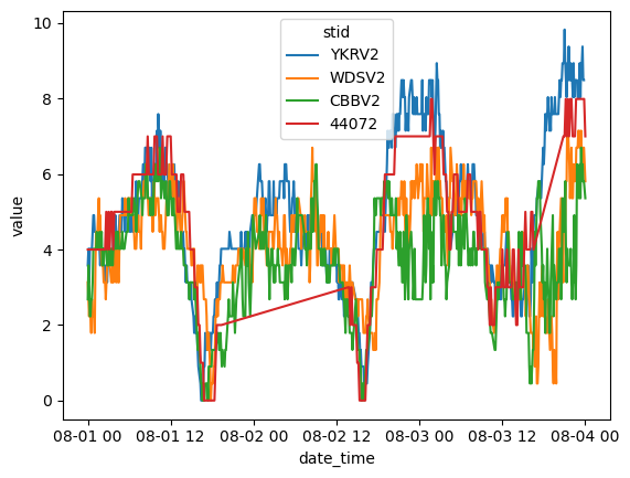
sns.lineplot(
    df.filter(variable="wind_speed"),
    x="date_time",
    y="value",
    hue="stid",
)

[5]:

<Axes: xlabel='date_time', ylabel='value'>

../../_images/user_guide_gallery_winds-chesapeake-bay_5_1.png

[6]:

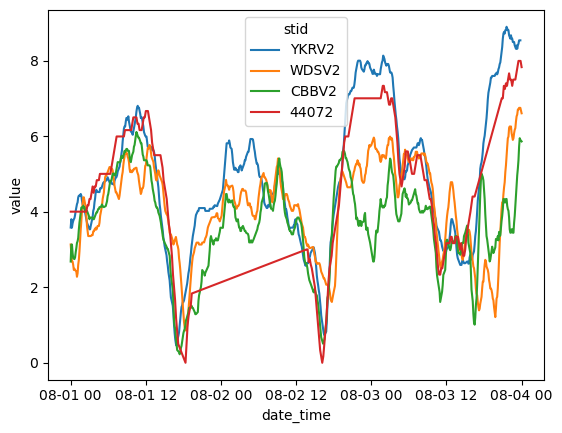
# Compute 60-min average wind speed

df_smoothed = (
    df.filter(variable="wind_speed", sensor_index=1)
    .sort("date_time")
    .rolling("date_time", period="60m", group_by="stid")
    .agg(pl.col("value").mean())
)

sns.lineplot(
    df_smoothed,
    x="date_time",
    y="value",
    hue="stid",
)

[6]:

<Axes: xlabel='date_time', ylabel='value'>

../../_images/user_guide_gallery_winds-chesapeake-bay_6_1.png

Pivot#

Let’s focus on one station and pivot the data to get variables in columns

[7]:

stid = "CBBV2"

a = (
    df.filter(stid=stid)  # Only focus on one station
    .synoptic.pivot()  # Pivot variable values into columns
    .synoptic.with_wind_uv()  # compute u and v wind component
)
a

[7]:

shape: (613, 10)

date_time	stid	latitude	longitude	elevation	wind_direction	wind_speed	wind_gust	wind_u	wind_v
datetime[μs, UTC]	str	f64	f64	f64	f64	f64	f64	f64	f64
2017-08-01 00:00:00 UTC	"CBBV2"	36.96667	-76.11333	0.0	139.0	2.68	4.91	-1.758238	2.022622
2017-08-01 00:06:00 UTC	"CBBV2"	36.96667	-76.11333	0.0	133.0	3.58	4.91	-2.618246	2.441554
2017-08-01 00:12:00 UTC	"CBBV2"	36.96667	-76.11333	0.0	138.0	3.13	4.47	-2.094379	2.326043
2017-08-01 00:18:00 UTC	"CBBV2"	36.96667	-76.11333	0.0	140.0	2.23	4.02	-1.433416	1.708279
2017-08-01 00:24:00 UTC	"CBBV2"	36.96667	-76.11333	0.0	146.0	2.23	3.58	-1.247	1.848754
…	…	…	…	…	…	…	…	…	…
2017-08-03 23:30:00 UTC	"CBBV2"	36.96667	-76.11333	0.0	166.0	5.81	7.15	-1.405566	5.637418
2017-08-03 23:36:00 UTC	"CBBV2"	36.96667	-76.11333	0.0	166.0	6.26	7.59	-1.514431	6.074051
2017-08-03 23:42:00 UTC	"CBBV2"	36.96667	-76.11333	0.0	164.0	5.81	6.7	-1.601453	5.58493
2017-08-03 23:48:00 UTC	"CBBV2"	36.96667	-76.11333	0.0	166.0	5.81	7.15	-1.405566	5.637418
2017-08-04 00:00:00 UTC	"CBBV2"	36.96667	-76.11333	0.0	173.0	5.36	7.15	-0.65322	5.320047

[ ]:

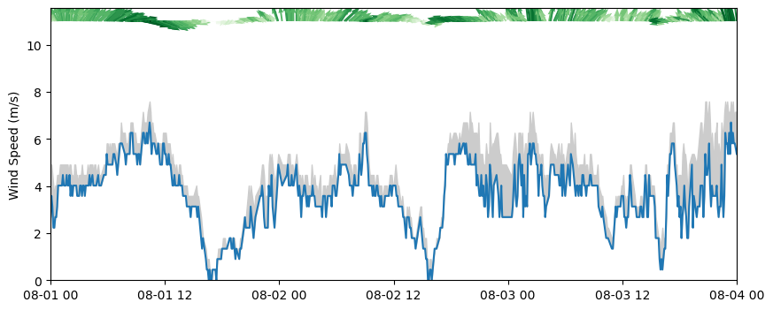
fig, ax = plt.subplots(1, 1, figsize=(10, 4))

ax.fill_between(a["date_time"], a["wind_speed"], a["wind_gust"], color=".8")
ax.plot(a["date_time"], a["wind_speed"], color="tab:blue")

ax.quiver(
    a["date_time"],
    a["wind_speed"] * 0 + 11,
    a["wind_u"],
    a["wind_v"],
    a["wind_speed"],
    cmap="Greens",
)

ax.set_ylim(ymin=0)
ax.set_xlim(a["date_time"].min(), a["date_time"].max())
ax.set_ylabel("Wind Speed (m/s)")

Text(0, 0.5, 'Wind Speed (m/s)')

../../_images/user_guide_gallery_winds-chesapeake-bay_9_1.png

[12]:

# Rolling
rolling_60m = a.rolling("date_time", period="60m", group_by="stid").agg(
    pl.col("wind_speed", "wind_u", "wind_v").mean(), pl.len()
)
rolling_60m

[12]:

shape: (613, 6)

stid	date_time	wind_speed	wind_u	wind_v	len
str	datetime[μs, UTC]	f64	f64	f64	u32
"CBBV2"	2017-08-01 00:00:00 UTC	2.68	-1.758238	2.022622	1
"CBBV2"	2017-08-01 00:06:00 UTC	3.13	-2.188242	2.232088	2
"CBBV2"	2017-08-01 00:12:00 UTC	3.13	-2.156954	2.263406	3
"CBBV2"	2017-08-01 00:18:00 UTC	2.905	-1.97607	2.124625	4
"CBBV2"	2017-08-01 00:24:00 UTC	2.77	-1.830256	2.06945	5
…	…	…	…	…	…
"CBBV2"	2017-08-03 23:30:00 UTC	5.363	-1.410243	5.112953	10
"CBBV2"	2017-08-03 23:36:00 UTC	5.721	-1.375518	5.527575	10
"CBBV2"	2017-08-03 23:42:00 UTC	5.944	-1.356663	5.776031	10
"CBBV2"	2017-08-03 23:48:00 UTC	5.899	-1.293414	5.747878	10
"CBBV2"	2017-08-04 00:00:00 UTC	5.858889	-1.187041	5.729993	9

[ ]:

# Group_by_dynamic
grouped_60m = a.group_by_dynamic(
    "date_time",
    every="60m",
    group_by="stid",
    include_boundaries=True,
).agg(pl.col("wind_speed", "wind_u", "wind_v").mean(), pl.len())

grouped_60m

shape: (73, 8)

stid	_lower_boundary	_upper_boundary	date_time	wind_speed	wind_u	wind_v	len
str	datetime[μs, UTC]	datetime[μs, UTC]	datetime[μs, UTC]	f64	f64	f64	u32
"CBBV2"	2017-08-01 00:00:00 UTC	2017-08-01 01:00:00 UTC	2017-08-01 00:00:00 UTC	3.038	-1.724122	2.460743	10
"CBBV2"	2017-08-01 01:00:00 UTC	2017-08-01 02:00:00 UTC	2017-08-01 01:00:00 UTC	4.11	-0.219624	4.065872	10
"CBBV2"	2017-08-01 02:00:00 UTC	2017-08-01 03:00:00 UTC	2017-08-01 02:00:00 UTC	3.889	0.945665	3.724923	10
"CBBV2"	2017-08-01 03:00:00 UTC	2017-08-01 04:00:00 UTC	2017-08-01 03:00:00 UTC	3.888	1.843056	3.403024	10
"CBBV2"	2017-08-01 04:00:00 UTC	2017-08-01 05:00:00 UTC	2017-08-01 04:00:00 UTC	4.1325	2.376548	3.363512	8
…	…	…	…	…	…	…	…
"CBBV2"	2017-08-03 20:00:00 UTC	2017-08-03 21:00:00 UTC	2017-08-03 20:00:00 UTC	3.888	-2.652406	2.802274	10
"CBBV2"	2017-08-03 21:00:00 UTC	2017-08-03 22:00:00 UTC	2017-08-03 21:00:00 UTC	4.023	-2.738462	2.934508	10
"CBBV2"	2017-08-03 22:00:00 UTC	2017-08-03 23:00:00 UTC	2017-08-03 22:00:00 UTC	3.889	-2.130629	3.161591	10
"CBBV2"	2017-08-03 23:00:00 UTC	2017-08-04 00:00:00 UTC	2017-08-03 23:00:00 UTC	5.908889	-1.237639	5.772571	9
"CBBV2"	2017-08-04 00:00:00 UTC	2017-08-04 01:00:00 UTC	2017-08-04 00:00:00 UTC	5.36	-0.65322	5.320047	1

[ ]:

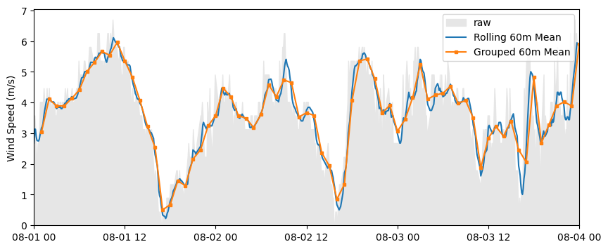
fig, ax = plt.subplots(1, 1, figsize=(10, 4))

ax.fill_between(a["date_time"], a["wind_speed"], color=".9", label="raw")

ax.plot(
    rolling_60m["date_time"],
    rolling_60m["wind_speed"],
    color="tab:blue",
    label="Rolling 60m Mean",
)

# I'm using `_upper_boundary` as the time value which says "at this
# time, the average wind speed for the previous hour was 'x'".
ax.plot(
    grouped_60m["_upper_boundary"],
    grouped_60m["wind_speed"],
    color="tab:orange",
    label="Grouped 60m Mean",
    marker="s",
    markersize=3,
)

ax.set_ylim(ymin=0)
ax.set_xlim(a["date_time"].min(), a["date_time"].max())
ax.set_ylabel("Wind Speed (m/s)")

ax.legend()

<matplotlib.legend.Legend at 0x7ff511d3a600>

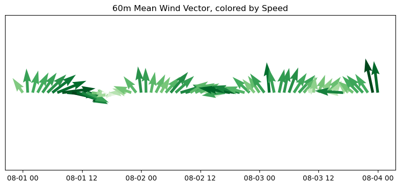
../../_images/user_guide_gallery_winds-chesapeake-bay_12_1.png

[47]:

# Plot quiver

fig, ax = plt.subplots(1, 1, figsize=(10, 4))

ax.quiver(
    grouped_60m["date_time"],
    grouped_60m["wind_speed"] * 0,
    grouped_60m["wind_u"],
    grouped_60m["wind_v"],
    grouped_60m["wind_speed"],
    cmap="Greens",
)

ax.set_ylim(-1, 1)
ax.set_title("60m Mean Wind Vector, colored by Speed")

ax.set_yticks([])

[47]:

[]

../../_images/user_guide_gallery_winds-chesapeake-bay_13_1.png